Reliability Trials
The need for trials is the most drastic situation for a system’s reliability rating: no data nor return on experience nor quantitative database is available, and/or the system is mechanical. It is also very useful for reliability growth once the system in service, to monitor the actual reliability of the system or a sub system. In these cases, you definitely need to proceed to a trial. Now the question is, which one is the most adapted for you? Let’s see.
What are the different trial Types?
Various types of trials cater to different needs or situations:
- RDGT (Reliability Development Growth Testing): Employed during the development phase, using the Duane Model.
- RQT (Reliability Qualification Testing) & PRAT (Product Reliability Acceptance Testing): These tests assess product compliance with reliability objectives through sequential testing.
- ESS (Environmental Stress Screening): trials conducted under significantly harsher conditions than normal, utilizing Accelerated Trials and the Arrhenius law.
What are the different reliability laws?
Knowing the failure law gives an insight about the system’s health or the system’s type of degradation. Knowing the law allows to determine the appropriate decision criteria, which are unique for each law.
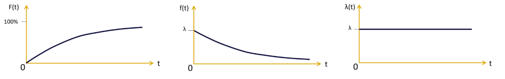
Exponential Law
The exponential law is the most widely used degradation law in RAMS for electric, electronic and programmable electronic systems, because it represents well their failure, and it is very convenient for calculation realization. Indeed, it is very convenient for the calculation of complex systems with many components, if they all follow the exponential law, because if all the components follow the exponential law, the system will also follow the exponential law. That’s because the only parameter to deal with is the failure rate, and it is constant.
Normal Law
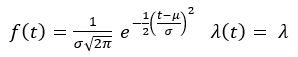
and F(t) is the integration of f(t). Its detailed expression would not help further comprehension.
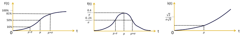
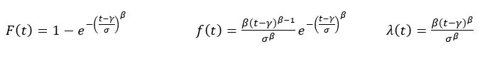
Weibull Law
The Weibull distribution is considered convenient for modeling a wide range of real-world phenomena due to its flexibility and ability to describe various shapes of probability density functions (PDFs). Here are some reasons why the Weibull distribution is often used and considered convenient:
The Weibull distribution can take on different shapes, making it versatile for modeling a variety of failure patterns. It can model increasing, decreasing, and constant hazard rates, which allows it to describe different types of reliability characteristics observed in practice.
The distribution has two parameters, shape (β) and scale (sometimes noted σ as an analogy with the normal law, or often η). These parameters provide flexibility in fitting the distribution to data with different characteristics. By adjusting these parameters, the Weibull distribution can closely match the observed data.
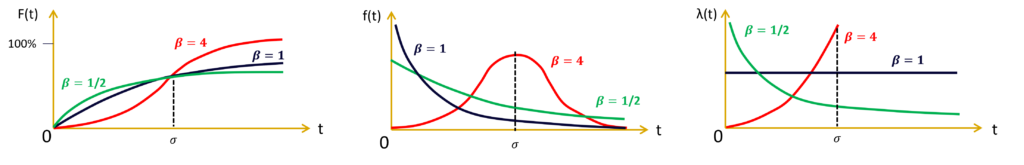
The shape parameter (β) in the Weibull distribution has an intuitive interpretation. When β >1, the hazard rate increases over time (early failure period). When β =1, the hazard rate is constant (useful for modeling random failures). When β <1, the hazard rate decreases over time (aging or wear-out period). It is widely used in trials analysis or reliability growth on service to determine on which part of the bathtub curve. Indeed:
- When β >1: This indicates that the hazard rate increases over time. In the early life of a system or component, the failure rate tends to rise. This is often associated with the presence of defective parts or initial manufacturing issues, leading to a higher likelihood of early failures. It corresponds to the “infant mortality” or “early failure” phase of the bathtub curve.
- When β =1: This implies a constant hazard rate. The failure rate remains constant over time, indicating a random or constant failure pattern. It corresponds to the “random failure” or “useful life” phase of the bathtub curve.
- When β <1: This indicates that the hazard rate decreases over time. As the system ages, the likelihood of failure decreases. It is often associated with wear-out or aging mechanisms. It corresponds to the “aging” or “wear-out” phase of the bathtub curve.
When the shape parameter (β) is greater than 1, the Weibull distribution tends to resemble a normal distribution, especially for larger values of β. In this case, the probability density function (PDF) of the Weibull distribution becomes more symmetric, and the shape of the distribution approaches a bell curve. The distribution becomes less skewed, and its tail behavior becomes more similar to that of a normal distribution. As β increases, the Weibull distribution becomes increasingly close to a normal distribution, making it a multipurpose distribution that can model a wide range of shapes.
How to associate the appropriate distribution to trial data?
Determining the appropriate probability distribution for trial data involves several steps, and statistical analysis can help identify the distribution that best fits the observed data. The details given help understand the approach, but it can be processed automatically by your favorite trial or reliability software.
Let’s take an example:
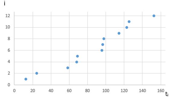
We consider 12 roll bearings, tested continuously, and we report their MTTF (ti).
i | ti (h) |
1 | 11.2 |
2 | 22.9 |
3 | 57 |
4 | 69.6 |
5 | 70.2 |
6 | 97.3 |
7 | 98.1 |
8 | 99.9 |
9 | 115.2 |
10 | 126.6 |
11 | 154.1 |
12 | 175.2 |
First, plot the data
Create visual representations of the data using histograms, cumulative distribution plots, or probability plots. These visualizations can provide initial insights into the distributional characteristics of the data.
Compare with Known Distributions
The first law to compare the data with is the Weibull law, whose shape can adapt to most of the reliability laws.
The Kolmogorov Smirnov test is the most common statistical test which allows to compare the appearance of trial data with a reference law. It can be done with a table. Let’s take back the upper example:
It is considered the start of the tests are at t=0, so γ=0.
I is the classification in the right time order (1 is the first failure 12 is the last failure)
Ti is the time when the failure occurred
is the estimated value of percentage of survivors, with a corrective bias to better represent the Weibull law (it is not necessary to understand the formula), and n is the total number of tested units here n=12.
The two following columns are intermediate calculation to trace the adequation regression curve.
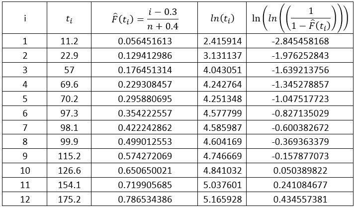
The regression line obtained with the fourth column in X-axis and the fifth column in Y-axis:
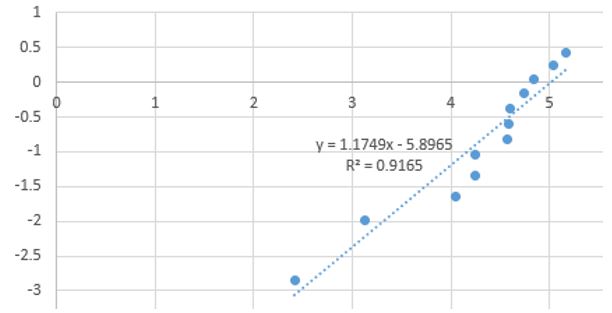
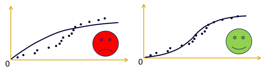
If the determination coefficient R^2 > 0.9, meaning that at least 90% of the regression determines the trial data distribution, the trial data can be associated with the tested law. In this case, our trial data fit with the Weibull distribution.
Now we can determine the Weibull parameters with the obtained correlation affine function with the form y=ax+b with a = 1.1749 and b = -5.8965 :
The directing coefficient a determines the value of β. Here β = a = 1.1749
And σ can be determined so : σ = exp(-b/β) = exp(5.8965/1.1749) = 151.22 hours
We can conclude, as β is slightly above 1, that the distribution is close to the exponential one, but an ageing factor is visible and makes the failure rate increase through time. It is actually common on mechanical components, much more subject to wear than electronical components, due to material friction.
If the determination coefficient with the line is under 0.9, it means that the distribution does not follow the Weibull law, and other adequation tests with other laws shall be performed. Fortunately, common reliability software does that automatically, and will give in output the best match, after performing every test.
How to determine the failure rate from a trial?
Three main cases are commonly encountered:
- Completed trials: the trials are still running until all the tested components are failed.
- Truncated trials: the trials are stopped when a certain time is reached, or the trials are still ongoing, but a first estimation can be made without needing all the failures from having failed.
- Censored trials: the trials are stopped right after the failure of a certain number of components.
For each case, here is how failure rates are estimated:
Truncated trials:
- If the components are not replaced once they are failed, the cumulated time of trial, noted τ is τ = t1 + t2 + t3 + … + tr+ (N-r)T with r the number of failed components, N the total number of components, and T the duration of the test.
- If the components are replaced once they are failed, the cumulated time of trial, is τ = N*T with N the total number of components, and T the duration of the test.
- The estimated failure rate
(the top ^ means it is an estimated value from observed values) is
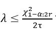
- The confidence interval for the failure rate is:
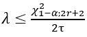
for unilateral limit, or
for bilateral limit.
Censored trials:
- If the components are not replaced once they are failed, the cumulated time of trial, noted τ is τ = t1 + t2 + t3 + … + tr+ (N-r)tr with r the number of failed components, and N the total number of components.
- If the components are replaced once they are failed, the cumulated time of trial, is τ = N* tr with N the total number of components, and tr the time the last component to fail before the end of the test came to fail (equivalent to the duration of the test).
- The estimated failure rate
is
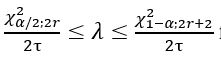
- The confidence interval for the failure rate is:
for unilateral limit, or
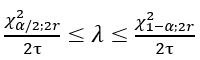
for bilateral limit.